Paired t test compares means of two observations recorded from a single unit or individual. Examples of such "paired" observations can be
1. Observations recorded at different times (Pre-test and Post-test scores) from same individuals
2. Observations recorded under two different conditions (Resting pulse rate and during exercise pulse rate)
3. Observations recorded from two halves of an individul or unit (e.g. Fairness in right half and left half of face).

Steps:

1. Null hypothesis and Alternate Hypothesis

Null Hypothesis

A. Two tailed test: Average difference in paired observations is equal to average expected difference. OR Average difference in paired observations is not significantly different than average expected difference.

B. One tailed test: (Right tailed): Average difference in paired observations is not more than average expected difference. OR Average difference in paired observations is equal to or less than average expected difference.

C. One tailed test: (Left tailed): Average difference in paired observations is not less than average expected difference. OR Average difference in paired observations is equal to or more than average expected difference.

 Alternate Hypothesis

A. Two tailed test: Average difference in paired observations is significantly different than average expected difference.

B. One tailed test: (Right tailed): Average difference in paired observations is significantly more than average expected difference.

C. One tailed test: (Left tailed): Average difference in paired observations is significantly less than average expected difference.

2. Calculate Test statistics t

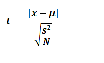
where t is the test statistics,
x̄ = Average difference in paired observations,
μ = Average expected difference,
s = Standard deviation,
N = Sample Size

3. Calculate Degrees of freedom (df).

df= N - 1

4. Know p value from t table

5. Interpret

If p < = alpha, then reject Null hypothesis, and accept alternate hypothesis.

If p > alpha, then the study has failed to reject Null hypothesis. So accept Null hypothesis.

---

Confidence Intervals

1. For two tailed test:

100 - alpha % confidence interval = x̄ ± critical_t_value * SE _mean
where critical_t_value is the t table value corrsponding to 2 tailed test, given alpha and degrees of freedom.
SE _mean = sqrt (s² / N)

1. For one tailed test:

A. Right tailed test (AH = Sample mean is significantly more than hypothesized mean)

100 - alpha % confidence interval = x̄ - critical_t_value * SE _mean to infinity.
where critical_t_value is the t table value corrsponding to 1 tailed test, given alpha and degrees of freedom.

B. Left tailed test (AH = Sample mean is significantly less than hypothesized mean)

100 - alpha % confidence interval = minus Infinity to x̄ + critical_t_value * SE _mean.
where critical_t_value is the t table value corrsponding to 1 tailed test, given alpha and degrees of freedom.

---

Example 1:

Following is the data of pre-test and post-test scores of 20 participants, recorded before and after a training session. Apply an approriate statistical test to test whether there is satistically significant difference in test scores, at alpha level of 5%.

Participant No	Pre-test score	Post-test score
1	10	15
2	12	13
3	9	11
4	8	10
5	15	11
6	13	14
7	11	11
8	12	12
9	10	9
10	8	15
11	9	10
12	10	9
13	8	8
14	10	10
15	9	12
16	10	11
17	10	12
18	10	14
19	10	12
20	10	14

These are 20 paired values, collected from 20 individuals. As N < 30 and population standard deviation is not known, appropriate statistical test will be "Paired t test."
Here,
x̄ = 1.45 (Average of difference between paired observations)
s = 2.4165
μ = 0 (Signifying, Null Hypothesis of no change in the paired observations)
N = 20
alpha = 5%
tails = 2 (significantly different) Putting above values at the respective places, we get the output as follows:

p = 0.0147. P value is statistically significant at given alpha level of 0.05 (5%). Average difference in paired observations is significantly different than average expected difference.

---

Example 2:

For above data, apply an approriate statistical test to test whether post-test score is significantly more than pre-test scores, at alpha level of 5%.

x̄ = 1.45 (Average of difference between paired observations)
s = 2.4165
μ = 0 (Signifying, Null Hypothesis of no change in the paired observations)
N = 20
alpha = 5%
tails = 2 (significantly different) Putting above values at the respective places, we get the output as follows

P = 0.0074. P value is statistically significant at given alpha level of 0.05 (5%). Average difference in paired observations is significantly more than average expected difference.

Avearge difference between pairs ± SD = 1.45 ± 2.4165
Expected difference = 0
Standard Error = 0.540345826762824
t = 2.68346663966455
df = 19
p = 0.00735202293048376 (One tailed)
Alpha = 0.05 (5 %). Critical t value = 1.7291327925089
95 % Confidence interval = 0.515670311649067 to ∞.