Simple linear regression is the simplest from
of linear regression in which the dependent variable is predicted using only one independent variable.
Multiple linear regression is a statistical technique used to predict dependent variable from multiple independent variables.
The general equation for multiple linear regression, when we have k number of independent variables, is
Y = β0 + β1*X1 + β2*X2 + ......βk*Xk
Where,
Y = Dependent variable
β0 = intercept or constant. It is the value of Y, when all X (independent) variables are 0.
β1 = regression coefficient for independent variable 1.
X1 = Value of first independent variable.
β2 = regression coefficient for independent variable 2.
X2 = Value of second independent variable.
Suppose, we want to estimate birth weight from 3 different independent variables - 1. Maternal Age 2. Maternal weight gain at 28 week, 3. Parity. The regression equation will be
BW = β0 + β1*Maternal_Age + β2*Maternal_Weight_Gain + β3*Parity
To estimate β coeficients for above example, we need to have a dataset as follows.
| ObsNo |
MAge |
MWG |
Parity |
BW |
| 1 |
25 |
6 |
1 |
2600 |
| 2 |
26 |
5 |
1 |
2500 |
| 3 |
22 |
6 |
0 |
2700 |
| 4 |
28 |
7 |
1 |
2800 |
| 5 |
32 |
6 |
2 |
2600 |
| 6 |
30 |
4 |
1 |
2200 |
| 7 |
31 |
5 |
1 |
2300 |
| 8 |
32 |
8 |
1 |
2800 |
| 9 |
32 |
4 |
2 |
2400 |
we can apply MLR using above dataset as follows:
Here, Number of Independent variables = 3. We can enter variable names and all 9 observations in the table as shown below.
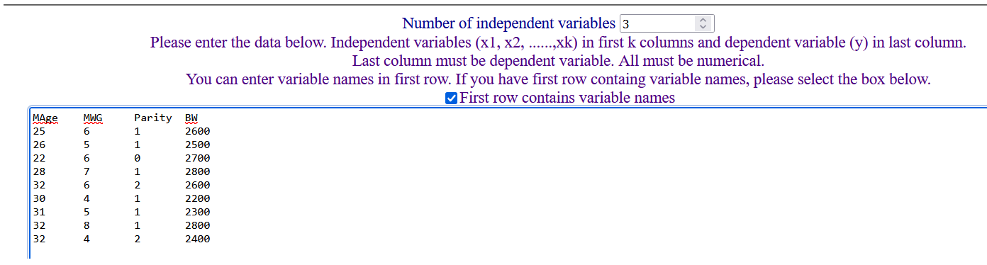 (The above data can be directly copied from excel and pasted in the text box.)
After providing significance level of say 5%, we can click on "Run Analysis" to get following output.
(The above data can be directly copied from excel and pasted in the text box.)
After providing significance level of say 5%, we can click on "Run Analysis" to get following output.
Descriptive.
| Variable | Mean | Standard Deviation | N |
|---|
| MAge | 28.6667 | 3.6401 | 9 |
| MWG | 5.6667 | 1.3229 | 9 |
| Parity | 1.1111 | 0.6009 | 9 |
| BW | 2544.4444 | 212.7858 | 9 |
Above table gives mean and standard deviations of three independent variables and dependent variable.
ANOVA.
| Model | Sum of Squares | df | Mean Sum of Squares | F | p |
|---|
| Regression | 336022.9119 | 3 | 112007.6373 | 21.3761 | 0.0028 |
|---|
| Residual | 26199.3103 | 5 | 5239.8621 |
|---|
| Total | 362222.2222 | 8 | |
|---|
Above table shows that F statistics is significant (p = 0.0028, p < 0.05). It means that these three IDVs can predict BW significantly better than mere mean of the BW.
Regression Sum of Squares (SSQRegression) is calculated using following formula.
SSQRegression = Σ (Ŷi - Ȳ)2
Ŷi = Predicted value of Y for ith observation, using regression equation. (Pronounced as Y hat).
Ȳ = Mean of all Y observed values.
SSQResidual = Σ (Yi - Ŷi)2
Where, Yi = Observed Y value for ith observation.
Coefficients
| Independent Variable | Coefficients | Standard Error of Coefficient | Standardized Coefficients | t | p | Confidence interval LB | Confidence interval UB |
|---|
| Constant | 2379.1034 | 272.4433 | | 8.7325 | 0.0003 | 1678.7656 | 3079.4413 |
| MAge | -30.8483 | 11.0682 | -0.5277 | -2.7871 | 0.0386 | -59.2999 | -2.3966 |
| MWG | 156.2345 | 20.4388 | 0.9713 | 7.644 | 0.0006 | 103.6949 | 208.774 |
| Parity | 147.8966 | 69.2617 | 0.4177 | 2.1353 | 0.0858 | -30.1463 | 325.9394 |
Above table shows β coefficients for three independent vaiables, its standard error, t value and significance. If β coefficient is significant, it means it is significantly different than 0, and its confidence interval will not include 0. From this table, we can derive regression equation as follows.
BW = 2379.1034 + (-30.8483)*MAge + 156.2345*MWG + 147.8966*Parity.
All coeffcients, except for parity, are significant.
Interpretation: The coefficient for maternal age is - 30.8483. What does it mean? It means, with every unit increase in age of the mother, there is decrease (negative sign) in birth weight by an amount of 30.8483, when other independent variables are kept constant.
Model Summary
| Model | R | R2 | Adjusted R2 | Std error |
|---|
| Enter (All IDV) | 0.9632 | 0.9277 | 0.8843 | 72.3869 |
|---|
Above table shows R, R squared and Adjusted R squared. R squared is calculated from ANOVA table using following formula.
R2 = (Regression Sum of Square) / (Total Sum of Squares)
Adjusted R2 = 1 - [(1 - R2) * (N - 1) / (N - k - 1)]
Where, N = Sample Size, k = Number of independent variables.
Here, adjusted R2 = 0.8843 means, 88.43% variation in the birth weights can be explained by above three independent variables.
As R2 and adjusted R2 can "measure" the combined effect of IDVs on DV, these are also called as measures of effect size. Other measures of effect size are
η2, f2, and f. These are interchangable, and can be calculated as follows.
η2 = R2
f2 = R2/ (1 - R2)
f = SQRT(f2)
f2 = η2/ (1 - η2)
-------------------
Here, first column specifies model method as "Enter". It means all the IDVs are used simulteneously in the analysis. (Other model methods are Stepwise, Remove, Forward, Backward.
In these types of methods IDVs are entered or removed in steps depending upon significance of its beta coefficients.)
MLR requires some assumptions to be satisfied by the data.
1. Dependent variable (continuos) should have fair linear correlation with each of the independent variables.
2. Multicollinearity should not be there.
3. Outliers (extreme Y observations) and High leverage values (extreme X observations) should be rechecked.
4. High influential points (observations which can substantially change beta coefficients and R square values) should be rechecked.
5. Residuals should be independent. (Not autocorrelated)
6. Homoscedasticity (equal variance) of residuals at all levels of predicted values.
7. Residuals should be normally distributed.
Assumptions testing
1. Dependent variable should have fair linear correlation with each of the independent variables.
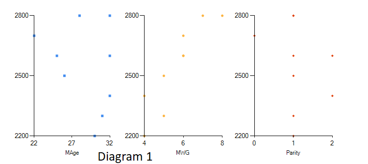
This assumption can be tested simply by looking at the scatter diagrams of dependent variable with eachof independent variables.
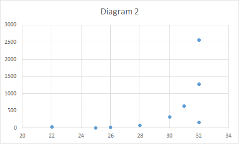
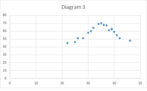
The scatter diagram should show a linear pattern (Diagram 1), or at least it should not show any other pattern like exponential pattern. (diagram 2) or curvilinear pattern(diagram 3)
Actions or remedies for non-linear relationship:
1. If exponential relationship: Use log values as variables. This will bring down the relationship to linear scale.
2. If relationship is curvilinear: Use quadratic regression.
3. You can add another variable, square of the IDV, i. e. X2, as a separate IDV.
4. Drop the IDV.
2. Multicollinearity should not be there.
Multicollinearity means there is high correlation between independent variables.
If independent variabls are correlated with each other, it causes inerpretations very difficult. (See above - interpretation of coefficients). Each coefficient tells about an increase in dependent variable
with unit increase in corresponding independent variable, when other IDV are kept constant. But if there is correlation amongst IDV, then other IDV can not be kept constant, making interpretations very difficult. Multicollinearity also increases the variance, and can make the coefficients non-significant. Lastly, multicollinearity can reverse the sign of a coefficient. It means when DV is expected to increase with increase in IDV, its beta coefficient can be negative, if the IDV is
correlated with other IDV.
Multicollinearity can be checked by
A. Correlaion coeficients between IDV.
Correlogram shows the correlation coefficients (r), between the variables.
In this correlogram table, if correlation coefficient between any two independent variables is > 0.8, these variables should be checked for multicollinearity.
B. Eigen values and Condition Index
Interpretation: If eigen values are very close to 0 (< 0.01) OR condition index > 30, then harmful multicollinearity is present.
C. Variance Inflation Factor (VIF) and Tolerance
VIF for each IDV (VIFi) is calculated by following formula.
VIFi = 1 / ( 1- Ri2)
Where, Ri2 is the R2 of the regression in which ith IDV is used as dependent variable, and remaining k-1 IDVs are used as IDVs.
In other words, to calculate VIF for maternal age in above example, we will use maternal age as dependent variable and remaining two (parity and MWG) as independent variables, run MLR and calculate Ri2
Then using above formula, it is easy to calculate VIFi. Tolerance is just reciprocal of the VIF.
If VIF > 10 OR Tolerance < 0.1, then harmful multicollinearity, related to those independent variables, is present.
Actions or remedies for multicollinearity:
1. If two or more IDVs are correlated with each other, compute a single IDV using all such IDVs, taking their averages, sums etc.
2. If this is not possible, then use alternate statistical technique such as ridge regression, lasso regression or principle component analysis.
3. Simply drop one of the IDV causing multicollinearity.
3. High leverage values (extreme X observations) and outliers (extreme Y observations) should be checked.
Extreme X values are called as leverage. Extreme Y values are called as outliers. Such leverage and outliers can adversely affect the coefficients and R2.
1. Please look carefully in the below diagram which shows two scatter plots. In the left plot, the red point (40, 60) has extreme X value, which is far away from the rest of the X values (between 22 and 35). So, it can be labelled as leverage. Right plot shows the scatter diagram and regression line after the observation is deleted.
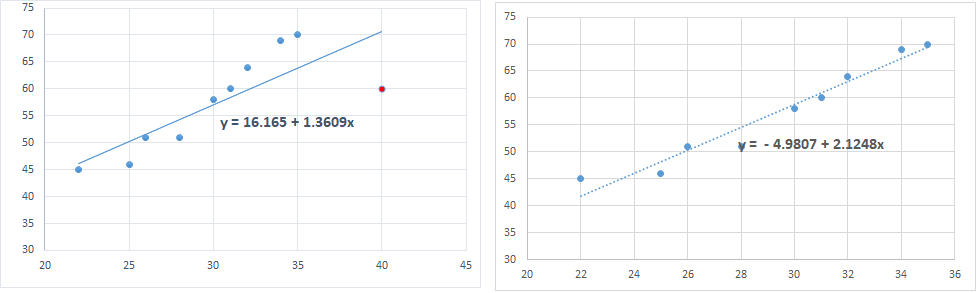
Not only the observation has extreme X value, it has also pulled the regression line towards itself. It has changed the slope of the regression line to 1.36 from otherwise 2.12, if the point was not there (Right scatter plot).
So, the observaion has substantially changed the beta coefficient as well as constant. This change in beta values because of the observation is called as DFBeta (Difference in Beta). We can also calculate standardized DFBeta. (See next assumption)
---------------------
2. Please look carefully in the below diagram which shows two scatter plots. In the left plot, the red point (34, 100) has extreme Y value, which is far away from the rest of the Y values (between 45 and 70). So, it can be labelled as an outlier. Right plot shows the scatter diagram and regression line after the observation is deleted.
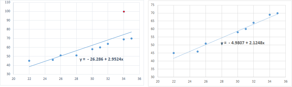
Not only the observation has extreme Y value, it has also pulled the regression line towards itself. It has changed the slope of the regression line to 2.95 from otherwise 2.12, if the point was not there (Right scatter plot).
So, the observaion has substantially changed the beta coefficient as well as constant. This change in beta values because of the observation is called as DFBeta (Difference in Beta). We can also calculate standardized DFBeta. (See next assumption)
------------------
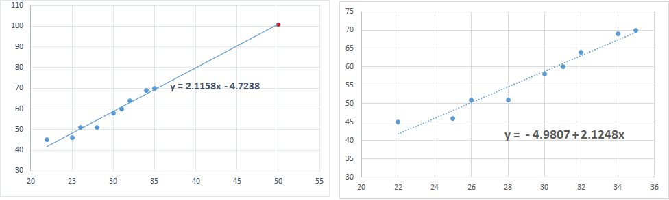
3. Please look carefully in the below diagram in which, the red point (50, 105) has extreme X and extreme Y value. So, it can be labelled as leverage as well as outlier. However it does not seem to affect the regression line. So leverage point and outlier need not necessarily affect the beta coefficients (need not be an influential
point).
----------------
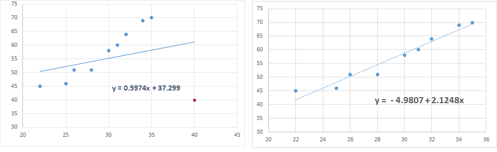
4. Please look carefully in the below diagram in which, the red point (40,
40) has extreme X and extreme Y value. So, it can be labelled as leverage as well as outlier. Aditionally it has significantly affected the regression line. Here, this leverage point and outlier is also an influential point.
----------------
-----------------------------------
If there is only one IDV, then extreme X observations can be identified by a scatter plot, as shown above. However, with more IDVs such multidimensional scatter plots can not be shown. In such situations, extreme X values are identified by "Leverage values" of every observation. This software provides "Leverage values" for all the observations entered in the analysis. The cut-off for leverage values is equal to [2 * (k + 1) / N].
If "Leverage value" of any of the observation is more than this cutoff value, then that observation has extreme X value.
Please note that SPSS gives leverage values which are less than above values by a margin of 1/N.
Total of leverage values provided by most of the softwares is (k+1). However SPSS gives total equal to k (No. of predictors).
(Leverage values here are equal to the diagonal elements of hat matrix.)
--------------------------
Second measure to identify leverage points is "Mahalanobis distance."
Mahalabonis distance (MD) for every observation is calculated using following formula.
MD = (N - 1) * (L - 1 / N)
L = Leverage value
To know whether MD is significant (indicating significant leverage observation), it's p value is calculated. MD follows chi-square distribution with k degrees of freedom.
So, it is easy to calculate p value for each Mahalanobis distance using chi-square tables. If p value of Mahalabonis distance < signficance level , then corresponding observation has significantly high leverage.
--------------------------
Third measure to identify leverage points is Cook's distance (CD). It is calculated using following formula.
CD = [L / (1 - L) 2] * (Y - Ŷ) 2 / [(k + 1) * MSQresidual]
Where, L = Leverage value, Ŷ (Y hat) is predicted value for the observation using regression equation,
MSQresidual = Residual Mean Sum of Squares (from ANOVA table)
The cut-off for Cook's distance is equal to 4 / N. If it is more than this cut-off , then corresponding observation has high leverage and it is also an outlier.
Actions or remedies for high leverage values or outliers
1. Check whether there is typo error for such observations.
2. If the observation additionally has high influence on DFFIT or DFBeta, then consider dropping the observation. However, before dropping the
observation you should ensure that the observation is really an "anomaly". Common-sense should prevail in this situation.
4. High influential points (observations which can substantially change beta coefficients and R square values) should be rechecked.
High influential points are those points, which because of there presence, can substantially change the beta coefficients, and so the predicted values for all observations. Such high influential points
can be identified by Difference in Fit (DFFit), and Difference in beta for every IDV (DFBeta) and their stadardized values.
A. DFFit (Difference in fit):
It is the change in predicted values when the model is run without the observation. (With sample size 1 less, after deleting the corresponding observation. )
So, DFFit for observation number 1, will be equal to the difference in predicted values with and without observation number 1.
B. Standardized DFFIt: DFFit / SE
C. DFBeta: (Difference in Beta Coefficients)
It is the change in coefficients when the model is run without the observation. (With sample size 1 less, after deleting the corresponding observation. )
D. Standardized DFBeta: DFBeta / SE
Interpretations:
If Standardized DFFit > 2 * SQRT [(k + 2) / (SS - k - 2)], then the observation has high influence in the model.
If Standardized DFBeta > 2 / N ^ 0.5, then the observation has high influence in the model.
It should be noted that, approxiately 5% of the observations can have standardized DFFit and standardized DFBeta values more than their respective cut-offs.
Actions or remedies for high influential points
1. Check whether there is typo error for such observations.
2. Consider dropping the observation after ensuring that the observation is really an "anomaly". Common-sense should prevail in this situation.
5. Residuals should be independent of each other. (They should not be auto-correlated)
Residuals (difference between actual Y and predicted Y) are said to be auto-correlated, if each residual is correlated with it's previous residual.
Auto-correlation in residuals is measured by Durbin Watson Statistics (DW), which is calculated as follows.
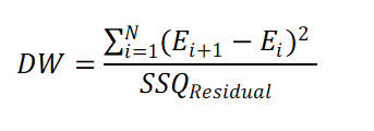
The Durbin Watson Statistics always have a value between 0 to 4. Values near to 2 are desirable to conclude that the residuals are not auto-correlated.
Practically, if DW statistics is between 1.5 and 2.5, we can say that the assumption of independent residuals is met.
(Please note that DW statistics depends on the sequencing of the observations Hence, it is possible that DW statistics with same but differently sorted observations can give different DW statistics.)
Actions or remedies for auto-correlated residuals.
1. Include lagged residuals as one of the predictors.
2. Statistcal techniques such as Cochrane-Orcutt Procedure, Hildreth-Lu Procedure or First Differences Procedure can be used.
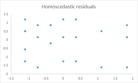
6. Homoscedasticity (equal variance) of residuals at all levels of predicted values.
Homoscedasticity of variance means variance is equal at all levels of predicted values.
Following scatter plot is the plot of standardized residuals on Y axis against standardized predicted values on X axis. .
This is typical example of homoscedasticity, as the variance of residuals is almost same at all levels of standardized predicted values.
------------------------------
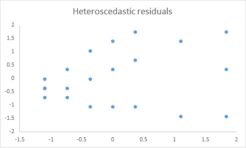
Following scatter plot shows that the variance of residuals goes on increasing from left to right.
This is typical example of heteroscedasticity.
T
Actions or remedies for heteroscedasticity of residuals.
1. Weighted least square method is used in regression.
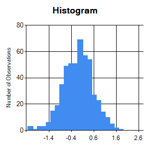
7. Residuals should be normally distributed.
Normally distributed residuals are typically tested by visual inspection of histrogram and Q-Q plot of residuals. Following diagram shows the histogram,
from which it can be inferred that the residuals are normally distributed.
------------------------------
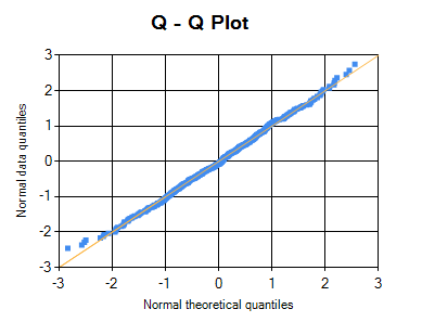
Following diagram is the Q-Q plot of the residuals.If residuals are normally distributed, then the points are very close to the central line.
Following Q-Q plot is a typical example of normally distributed residuals, as most of its points are very close to the central line.
--------------------------
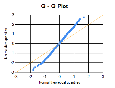
Following Q-Q plot of the residuals shows that residuals are not normally distributed, as many of its points are deviated from the central line.
T
Actions or remedies for heteroscedasticity of residuals.
1. Redo the regression after removing influential points.
2.
Transform IDVs into log scale, after visually inspecting and identifying the exponential curve for the IDVs.
A note on Dummy Variables
If any of the independent variables is categorical, then we need to create dummy variables for such categorical variable. How the dummy variables are created?
Suppose there are "k" different categories in that variable, then a total of "k-1" dummy variables are created, one each for a category, except for one which is used as the reference category.
For example, a categorical variable "smoking status" has three categories: Non_Smoker, Occassional_Smoker and Regular_Smoker. Here two dummy variables are created: Is_Occassional_Smoker, Is_Regular_Smoker.
Non_Smoker will be the reference category. In dummy variable "Occassional_Smoker"; value "1" will be assigned to Occassional smokers and rest of the persons will have value "0". Following table explains how dummy variables are created.
| Person No |
Smoking Status |
Dummy variables |
| Is_Occasional_Smoker |
Is_Regular_Smoker |
| 1 |
Occasional_Smoker |
1 |
0 |
| 2 |
Regular_Smoker |
0 |
1 |
| 3 |
Occasional_Smoker |
1 |
0 |
| 4 |
Regular_Smoker |
0 |
1 |
| 5 |
Regular_Smoker |
0 |
1 |
| 6 |
Non_Smoker |
0 |
0 |
| 7 |
Occasional_Smoker |
1 |
0 |
| 8 |
Non_Smoker |
0 |
0 |
| 9 |
Non_Smoker |
0 |
0 |
Please note that, the reference category (Non-Smoker) is represented by "0" s in all dummy variables.
This software automatically creates k-1 dummy variables for k categories in each of categorical variables.
Needless to say that, total number of independent variables are increased in this situation.
@ Sachin Mumbare