Two way ANOVA (Analysis of Variance) is applied to test how two independent variables affects a dependent variable.
For example, suppose you want to compare the marks scored by urban, rural and semi-urban students, you will have three different means to compare with each other.
Here, appropriate test of significance will be one way ANOVA. ("One way" - signifying only one independent variable, residence). Also, we can deduce that there are three levels (or categories or groups) withing this independent variable.
Now, suppose that, another independent variable is added i. e. Gender, in the study. Now, we have two independent variables, residence - having three levels and gender having two levels.
If our first independent varible - residence - has significant impact on scores, then
means scores of students from these three categories of residents will have significantly different scores. Similarly, if gender
has significant impact on scores, then means scores in two genders will be significantly different.
But, the impact of gender on three different categories of residences can be different, e. g. rural and urban students can experience different impact of gender!
So this is interaction effect.
In this situation, we want to test whether both independent variables have significant effect on the continuous variable, separately. Additionally, we may also want to test whether there is an interaction effect. Two way ANOVA is the test applied in this situation.
Assumptions
1. There are two categorical independent variables, with two or more levels / categories in each independent variable.
2. Dependent variable is continuous and normally distributed in all the possible combinations of two independent variable levels.
3. Samples are drawn using random sampling technique.
4. The observations are independent. There are no observations, which are in more than one group.
5. The variance in all the groups is same. (homogeneity
of variance / homoscedasticity). It can be tested by Levene's test of homogeneity of variance.
6. There are no outliers.
Steps:
1. Null hypothesis and Alternate Hypothesis
Null Hypothesis
A. The sample means for all categories in first independent variable (A) are equal . (x̄i = x̄j )
B. The sample means for all categories in second independent variable (B) are equal . (x̄i = x̄j )
C. There is no interaction between factors A and B.
Alternate Hypothesis
A. The sample means for at least two categories in first independent variable (A) are not equal . (x̄i≠ x̄j )
B. The sample means for at least two categories in second independent variable (B) are not equal . (x̄i ≠ x̄j )
C. There is significant interaction between factors A and B.
2. Calculate Sum of Squares for IDV A (SSA Between)
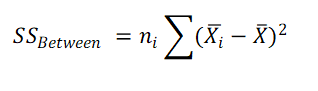
where ni is the sample size of category / group i in IDV A.
x̄ = Grand mean (Mean of all the observations)
x̄i = Mean of level (group) i for IDV A.
ni = Sample size in group i for IDV A.
3. Calculate Sum of Squares for IDV B (SSB Between)
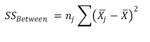
where nj is the sample size of level / category / group j in IDV B
x̄ = Grand mean (Mean of all the observations)
x̄j = Mean of level (group) j for IDV B.
nj = Sample size in group j for IDV B.
4. Calculate Sum of Squares Within (SSE) (Error)
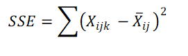
xijk = kth observation in group ij. (Observation from level i for IDV A and level j for IDV B)
x̄ij = Mean of group ij (Mean of observations from level i for IDV A and level j for IDV B).
5. Calculate Interaction Sum of Squares (SS AB)
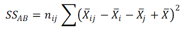
x̄ij = Mean of group ij (Mean of observations from level i for IDV A and level j for IDV B).
x̄i = Mean of group i from IDV A.
x̄j = Mean of group j from IDV B.
x̄ = Grand Mean (Mean of all the observations)
nij = Sample size in group ij.
6. Calculate Total Sum of Squares (SS T)
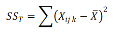
xijk = kth observation in group ij. (Observation from level i for IDV A and level j for IDV B).
x̄ = Grand mean
6. Calculate degrees of freedom
df_A = Degrees of freedom for IDV A= a - 1
df_B = Degrees of freedom for IDV B= b - 1
df_AB = Degrees of freedom interaction AB = (a -1) * (b - 1)
df_Error = Degrees of freedom for Error = N - a * b
df_total = Degrees of freedom Total = N -1
N = Grand Sample Size, a = Number of levels / groups / categories in IDV A, b = Number of levels / groups / categories in IDV B, IDV = Independent variable
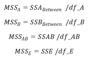
7. Calculate Mean Sum of Squares for IDV A, IDV B, interaction
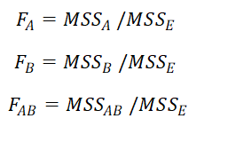
8. Calculate F value for IDV A, IDV B and interaction
6. Calculate p values, using F table for IDV A, IDV B and interaction AB.
7. Interpret all three p values
If, p < = alpha, then reject the respective Null hypothesis
If, p > alpha, then accept respective null hypthesis
8. Post hoc tests
If, p < = alpha, alternate hypothesis is accepted (at least two means are significantly different)
Which pair (or pairs) of means are significantly different is now identified by post hoc tests.
There are multiple post hoc tests available, out of which Benferroni and Tukey HSD are most commonly used.
Steps for applying two way ANOVA using this software
1. To apply two way ANOVA here, you need to arrange the data in three columns.
First row of the data can be used for variable names. First Column must be of dependent variable, which must be numerical. Second and third column
should be of independent variables 1 and 2. You can copy the data (in three columns in exact sequence as specified above), from any other file such as excel, and paste directly into the text box. Please do not include any other column (such as subject no / sr no etc).
2. Specify your choosen significance level or alpha (usually 5 or 1).
3. Specify the type of "Sum of Squares (SSQ) you want. There are three options availabale.
Most commonly used option is "Type III". You can select that default option of Type III. Other options are "Type I" and "Type II". Please see details about SSQ given at the bottom.
4. Click on "Run Test".
5. Following is example of input and output, with detailed description and explanation.
Suppose you want to compare mean systolic blood pressure in athletes participating in four different sports: Marathon, Football, Chess and Swimming. Also you want to add Gender as your second independent variable. Following is the data of athletes, with their respective systolic blood pressures, Sports and Gender. Please note that data is arranged in three columns with specified sequence.
| SBP |
Sports |
Gender |
| 136 |
Chess |
Male |
| 122 |
Chess |
Female |
| 118 |
Swimming |
Male |
| 110 |
Football |
Female |
| 140 |
Chess |
Male |
| 136 |
Chess |
Male |
| 120 |
Football |
Male |
| 128 |
Chess |
Male |
| 112 |
Football |
Female |
| 118 |
Swimming |
Female |
| 126 |
Swimming |
Male |
| 128 |
Marathon |
Male |
| 122 |
Football |
Male |
| 118 |
Football |
Female |
| 126 |
Swimming |
Male |
| 124 |
Football |
Male |
| 126 |
Chess |
Female |
| 116 |
Chess |
Female |
| 132 |
Chess |
Male |
| 114 |
Marathon |
Female |
| 118 |
Football |
Male |
| 134 |
Marathon |
Female |
| 120 |
Marathon |
Female |
| 114 |
Swimming |
Male |
| 128 |
Chess |
Male |
| 136 |
Chess |
Male |
| 120 |
Football |
Female |
| 120 |
Swimming |
Male |
| 128 |
Marathon |
Male |
| 128 |
Swimming |
Female |
| 126 |
Football |
Female |
| 118 |
Chess |
Male |
| 128 |
Chess |
Male |
| 116 |
Football |
Male |
| 120 |
Football |
Male |
| 124 |
Marathon |
Male |
| 120 |
Chess |
Female |
| 136 |
Chess |
Male |
| 120 |
Marathon |
Male |
| 112 |
Chess |
Female |
| 120 |
Swimming |
Female |
| 110 |
Marathon |
Female |
| 122 |
Swimming |
Female |
| 122 |
Chess |
Female |
| 118 |
Marathon |
Male |
| 130 |
Chess |
Female |
| 110 |
Chess |
Female |
| 126 |
Marathon |
Female |
| 122 |
Swimming |
Male |
| 124 |
Football |
Male |
| 124 |
Swimming |
Female |
| 150 |
Chess |
Male |
| 144 |
Chess |
Female |
| 116 |
Marathon |
Male |
| 118 |
Marathon |
Female |
| 114 |
Marathon |
Female |
| 120 |
Swimming |
Male |
| 120 |
Chess |
Male |
| 120 |
Swimming |
Female |
| 144 |
Chess |
Male |
You can copy and paste above data into excel sheet, to have it in the required format. Then from excel you copy and paste the data in the given textbox.
Select 5% as alpha and Type III model type for SSQ. Finally click on "Run Test".
Following are the results
Descriptive: Sports
| Category | Mean | SD | Sample Size |
| Chess | 128.8182 | 10.7554 | 22 |
| Swimming | 121.3846 | 3.863 | 13 |
| Football | 119.1667 | 4.7832 | 12 |
| Marathon | 120.7692 | 6.8575 | 13 |
Above table shows the mean SBP, SD and Number of study participants in four different sports.
Descriptive: Gender
| Category | Mean | SD | Sample Size |
| Male | 125.9394 | 8.6817 | 33 |
| Female | 120.5926 | 7.8214 | 27 |
Above table shows Gender wise mean SBP, SD and Number of study participants.
Descriptive: Both Independent Variables
| Chess | Swimming | Football | Marathon |
|---|
| Male | 133.2308 (13) | 120.8571 (7) | 120.5714 (7) | 122.3333 (6) |
| Female | 122.4444 (9) | 122 (6) | 117.2 (5) | 119.4286 (7) |
Above table shows Gender and Sports wise mean (Number of subjects)
ANOVA Table
| Sum of Squares (Type III) | df | Mean Sum of Squares | F | p | Partial eta squared |
| Between Groups (Sports) | 784.3749 | 3 | 261.4583 | 4.9603 | 0.0042 | 0.2225 |
| Between Groups (Gender) | 220.3904 | 1 | 220.3904 | 4.1811 | 0.046 | 0.0744 |
| Interaction (Sports * Gender) | 321.868 | 3 | 107.2893 | 2.0354 | 0.1203 | 0.1051 |
| Corrected model | 1685.9844 | 7 | 240.8549 | 4.5694 | 0.0005 | 0.3808 |
| Within Groups (Error) | 2740.949 | 52 | 52.7106 |
Above table shows the results of Two Way ANOVA. This table is the main output of the test. It shows Sum of Squares: SSQ(Type III) for each of the independent variable and interaction variable, degrees of freedom: df, Mean Sum of Squares (MSQ), F value, p and partial eta squared.
We are interested only in three rows. Two rows corresponding to two independent variables (Sports and Gender) and one row corresponding to interaction. (Rows with highlighted background)
First row, corresponding to IDV- Stay, shows that the F = 4.9603 and p = 0.0042. As p < 0.05. So we can infer that there is significant difference in at least two category means of SBP for different Sports.
Similary, for second row, corresponding to IDV- Gender, F=4.1811 and p=0.046, with similar interpretation of significant difference in at least two category means in Gender (Incidently there are only two means in Gender)
Partial eta square is the measure effect size, quantifying the variance explained by the independent variable, after excluding variance explained by other independent variable. Here partial eta squared for Sports is 0.2225, signifying that about 22.25% of variation in SBP can be explained by Sports.
Finally p value for interaction is 0.1203 (non-significant), indicating that there is no significant interaction of Sports and Gender for SBP.
So, we can infer that at least two means in Sports and at least two means in Gender are significanly different. For Gender, as there are only two means (for Males and Females), there is no issue in identifying such two menas. However, for IDV Sports, we need to apply post-hoc test to identify which means are significantly different. Most commonly used post hoc tests are Bonferroni test and Tuckey HSD test. Following are the results of the both the tests for IDV Sports.
Bonferroni test (Sports)
| Comparison between | Difference between means | Standard error | t | critical t | Bonferroni adjusted p | Confidence interval LB | Confidence interval UB |
| Mean:Chess AND Mean:Swimming | 7.4336 | 2.5398 | 2.9268 | 2.743 | 0.0304 | 0.467 | 14.4001 |
| Mean:Chess AND Mean:Football | 9.6515 | 2.6055 | 3.7043 | 2.743 | 0.0031 | 2.5048 | 16.7982 |
| Mean:Chess AND Mean:Marathon | 8.049 | 2.5398 | 3.1691 | 2.743 | 0.0154 | 1.0824 | 15.0155 |
| Mean:Swimming AND Mean:Football | 2.2179 | 2.9064 | 0.7631 | 2.743 | 1 | -5.7542 | 10.1901 |
| Mean:Swimming AND Mean:Marathon | 0.6154 | 2.8477 | 0.2161 | 2.743 | 1 | -7.1957 | 8.4265 |
| Mean:Football AND Mean:Marathon | -1.6026 | 2.9064 | 0.5514 | 2.743 | 1 | -9.5747 | 6.3696 |
We can see that p vaules for comparision between means of Chess and Swimming, Chess and Football, Chess and Marathon (three pairs of means) are significantly different. Thus, the Bonferroni test has identified three pairs of means which are significantly different than each other.
Following are the results of post hoc Tuckey HSD test
| Comparison between | Difference between means | Standard error | p | Confidence interval LB | Confidence interval UB |
| Mean: Chess AND Mean: Swimming | 7.4336 | 2.5398 | 0.0253 | 0.6919 | 14.1752 |
| Mean: Chess AND Mean: Football | 9.6515 | 2.6055 | 0.0028 | 2.7355 | 16.5675 |
| Mean: Chess AND Mean: Marathon | 8.049 | 2.5398 | 0.0132 | 1.3073 | 14.7906 |
| Mean: Swimming AND Mean: Football | 2.2179 | 2.9064 | 0.8706 | -5.4969 | 9.9328 |
| Mean: Swimming AND Mean: Marathon | 0.6154 | 2.8477 | 0.9964 | -6.9435 | 8.1743 |
| Mean: Football AND Mean: Marathon | -1.6026 | 2.9064 | 0.9458 | -9.3174 | 6.1122 |
Results are Tuckey HSD test are also similar to Bonferroni test.
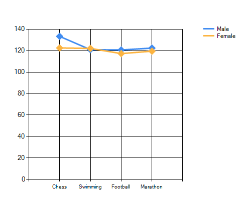
Above chart shows the Sports-wise means of SBP in two Genders. It can be seen that the lines for two genders are just crossing each other, suggesting a little bit of interaction.
However, just after crossing the lines are almost parallel, suggesting non-signficant interaction. If lines cross each other, and diverse apart, it suggests significant interaction.
How to report these findings:
A two-way ANOVA was performed to compare the effects of Sports in which a person indulged and Gender on Systolic Blood Pressure.
It revealed that there was significant difference in SBP between at least two group means in Sports (F=4.9603, df=3, p=0.0042). Post hoc Bonferroni test revealed that the means of SBP
for Chess players and Swimmers were significantly different (Bonferroni adjusted p = 0.467 ).
Similarly means of SBP in Chess players and Marathon runners (Bonferroni adjusted p = 0.0154 )
and those in Chess players and Football players (Bonferroni adjusted p =0.0031) were also significantly different.
Tukey’s HSD test also reveled similar findings.
The two-way ANOVA also revealed that there was significant difference between means of SBP in males and females (F=4.1811, p=0.046).
There was no significant effect of interaction between Sports and Gender (F=2.0354, p=0.1203).
@ Sachin Mumbare