ANOVA (Analysis of Variance) is applied to compare more than two independent sample means.
Assumptions
1. Dependent variable is continuous and normally distributed in all the groups.
2. Samples are drawn using random sampling technique.
3. The observations are independent. There are no observations, which are in more than one group.
4. The variance in all the groups is same. (homogeneity
of variance / homoscedasticity). It can be tested by Levene's test of homogeneity of variance.
5. There are no outliers.
6. There is one independent variable, which is nominal or ordinal, with more than two possible levels / categories.
Steps:
1. Null hypothesis and Alternate Hypothesis
Null Hypothesis
A. All the sample means are equal. (μi = μj)
Alternate Hypothesis
A. There are at least two means (at least a pair of means), which are different than each other. (μi ≠ μj)
Where μi and μj can be any two sample means.
2. Calculate Sum of Squares for Treatment (SS Between)
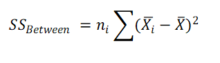
where ni is the sample size of group i,
x̄ = Grand mean (Mean of all the observations)
x̄i = Mean of group i
3. Calculate Sum of Squares Within (SS Error)
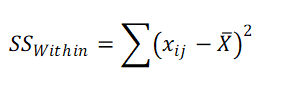
x̄ = Grand mean (Mean of all the observations)
xij = jth observation in group i.
4. Calculate Mean Sum of Squares for Treatment and Mean Sum of Squares for Error
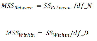
df_N = Degrees of freedom for Numerator = k - 1
df_D = Degrees of freedom for Denominator = N - k
N = Grand Sample Size, k = Number of groups
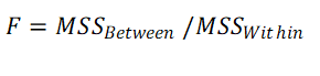
5. Calculate F value
6. Calculate p value, using F table
7. Interpret
If, p < = alpha, then reject the Null hypothesis
If, p > alpha, then accept null hypthesis
8. Post hoc tests
If, p < = alpha, alternate hypothesis is accepted (at least two means are significantly different)
Which pair (or pairs) of means are significantly different is now identified by post hoc tests.
There are multiple post hoc tests available, out of which Benferroni and Tukey HSD are most commonly used.
8. A. Benferroni
Multiple tests can increase the type I error rate. For example if n simulteneous t tests are used for an alpha of 0.05 for each test, then total alpha will be 1 - (1 - alpha)n.
So, if there are three means to be compared in ANOVA, we need to apply three different t tests. So total resultant alpha will be 1 -(1-0.05)3 = 0.142625, much more than intended 0.05.
Hence, an adjustment is done by applying t test for each pair with adjusted alpha of alpha / (total no. of tests applied).
{Alternately, the p value can be adjusted (Bonferroni adjusted p) by multiplying the p value got during each t test with total no. of tests to be applied.}
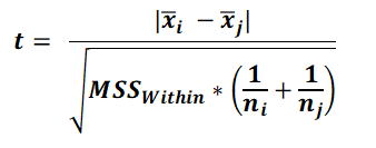
In Benferroni post hoc test, for each pair of means t statistics is calculated as follows.
The resultant p value is to be multiplied by no. of tests (No. of pairs), to get Bonferroni adjusted p value. Please that the degrees of freedom, while calculating p value, is equal to the df_D in applied ANOVA. If Bonferroni adjusted p value is less than the inended alpha, then the means in the pairs are significantly different.
If there are n groups, then total no. of tests (No. of pairs) will be n * (n - 1) / 2.
Confidence intervals for Bonferroni post hoc test
Critical t value is calculated using df = df_D and adjusted alpha (original alpha / no. of tests)
LB of CI = (x̄i - x̄j) - (critical t) * SE
UB of CI = (x̄i - x̄j) + (critical t) * SE
Here, SE = SQRT (MSBetween * (1/ni + 1/nj)
Please note that, SE is exactly equal to the denominator used for calculating t in above equation.
Example 1:
Random samples of 25 each from rural, semi-urban and urban students have shown mean IQ of 111.68 ± 5.4522, 102.48 ± 12.7381 and 102.40 ± 13.6626, respectively. Apply an approriate statistical test to test whether there is residence-wise significantly difference in IQ, at alpha level of 5%.
As there are more than two means to be compared, appropriate statistical test is ANOVA.
Here,
x̄ 1 = 111.68,
SD1 = 5.4522,
N1= 25
x̄ 2 = 102.48,
SD2 = 12.7381,
N2= 25
x̄ 3 = 102.40,
SD3 = 13.6626,
N3= 25
alpha = 5%
Putting above values at the respective places, we get the output as follows:
ANOVA Table
| Sum of Squares | df | Mean Sum of Squares | F | p |
|---|
| Between Groups | 1423.04 | 2 | 711.52 | 5.6373 | 0.0053 |
| Within Groups | 9087.6556 | 72 | 126.2174 |
| Total | 10510.6956 | 74 | |
Post-hoc test results.
Bonferroni correction.
| Comparison between | Difference between means | Standard error | t | critical t | Bonferroni adjusted p | Confidence interval LB | Confidence interval UB |
| Mean: 1 AND Mean: 2 | 9.2 | 3.1776 | 2.8952 | 2.4512 | 0.015 | 1.411 | 16.989 |
| Mean: 1 AND Mean: 3 | 9.28 | 3.1776 | 2.9204 | 2.4512 | 0.014 | 1.491 | 17.069 |
| Mean: 2 AND Mean: 3 | 0.08 | 3.1776 | 0.0252 | 2.4512 | 1 | -7.709 | 7.869 |
Post-hoc test results.
Tukey HSD.
| Comparison between | Difference between means | Standard error | p | Confidence interval LB | Confidence interval UB |
| Mean: 1 AND Mean: 2 | 9.2 | 3.1776 | 0.0137 | 1.5947 | 16.8053 |
| Mean: 1 AND Mean: 3 | 9.28 | 3.1776 | 0.0128 | 1.6747 | 16.8853 |
| Mean: 2 AND Mean: 3 | 0.08 | 3.1776 | 0.9997 | -7.5253 | 7.6853 |
As p = 0.0053 in ANOVA, p is significant. We can say that there are at least two means which are statistically significantly different than each other.
To find the pair (pairs), post hoc tests are applied.
Post hoc tests have shown that Mean 1 (rural) and Mean 2 (semi-urban) are significantly different.
Similarly, Mean 1 (rural) and Mean 3 (urban) are also significantly different.
However, Mean 2 (semi-urban) and Mean 3(urban) are not significantly different.
How to report ANOVA results:
One-way ANOVA was performed to compare mean IQ of students amongst various categories of their residence (rural, semi-urban and urban).
It revealed that there was significant difference in mean IQ between at least two category means. (F=5.6373, p=0053). Post hoc Bonferroni test revealed that the means IQ of rural and semi-urban students was significantly different (p=0.015). Similarly mean IQ of rural and urban students was also significantly different (p=0.014).
@ Sachin Mumbare