Meta-analysis of retrospective studies (effect size = Odds Ratio)


The meta-analysis can be done using following models.

1. Fixed effect model
2. Random effects model

Selection of appropriate model depends upon the heterogeneity amongst the included studies. (see below for details)


Fixed effect meta-analysis: Steps

1. Calculating / extracting effect size = OR (Odds ratio) for each included studies.

OR = ad/bc
(where a = number of exposed in cases, b= number of non-exposed in cases, c= number of exposed in controls , d= number of non-exposed in controls)

2. Calculating LogeOR for each included studies. (Log Odds Ratio base e)

3. Calculating Variance (V) and Standard Error of Log (OR)

Variance for ith study (Vi) = (1/a + 1/b + 1/c + 1/d)
SELog OR = sqrt(1/a + 1/b + 1/c + 1/d)

4. Calculating confidence intervals for Log (OR) and converting them to original scale for each study.

A. Confidence intervals for Log OR
LB CI = Log (OR) - Z1-α/2 * SE Log OR
UB CI = Log (OR) + Z1-α/2 * SE Log OR

B. Confidence intervals of OR
We can convert above confidence intervals into original scale by following formula.
OR = eLog OR

5. Weights (W) of each included studies under fixed effect model (inverse variance method)

Wi = 1/Vi

6. Summary Log OR (meta-analysis Log OR) under fixed effect model is calculated as follows


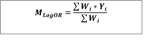
MALog OR = Summary Log OR
Wi= Weight for ith included study
Yi= Log OR for ith included study

7. Standard Error of MALog OR = 1/Σ Wi

Once summary Log OR and its standard error is calculated, it is fairly easy to calculate confidence intervals.
We can convert summary Log OR and its confidence intervals into original scale as described above under point 4(B).

8. Z value and p value.

Once summary Log OR and its standard error is calculated, it is fairly easy to calculate Z value and p value using normal distribution.
Z = MALog OR / Standard Error of MALog OR


If available data is Odds Ratio and its confidence interval, then log Odds Ratio is initially calculated. SE of log Odds Ratio is calculated from UB and LB of confidence intervals, as follows.

SELog OR = (UBLog OR - Log OR) / Z1−α/2
It can be also calculated as follows
SELog OR = (Log OR - LBLog OR) / Z1−α/2
Variance (V) = SE2


Measures of heterogeneity

Not all included studies are homogeneous with respect to characteristics of participants such as age, gender, geo-environmental factors, other socio-demographic factors, selection criteria for cases etc. When these differences are present, variability in the study results is not just random, and the studies are considered as heterogeneous. This heterogeneity is quantified by following measures of heterogeneity.

1. Cochran's Q statistics

Q = Σ Wi * (Yi - M)2
Yi = Log OR for ith study
M = Summary Log OR (Meta-analysis Log OR)

Q statistics follows chi-square distribution with k - 1 degrees of freedom (k= number of included studies)
So, p value for Cochran's Q statistics can easily be calculated using chi square distribution.
Significant p value indicates that significant heterogeneity is present, and we should consider other methods of meta-analysis like random effects model or sub-group analysis or meta-regression.

2. Tau squared (τ2) statistics

τ2= (Q - (k -1)) / C
where,
C = Σ Wi - Σ Wi 2 / Σ Wi
Σ Wi = Sum total of weights of all included studies
Σ Wi2 = Sum total of squared weights of all included studies

3. I2 statistics

I2= 100 * (Q - (k -1)) / Q
I2 statistics is measured in percentage. I2 value of < 25% is considered as low heterogeneity, between 25 and 50 it is moderate and above 50% it is significant heterogeneity.

All above measures of heterogeneity provides a quantified measure, but they can not identify the factors causing heterogeneity.


Random effects model

If fixed effect meta-analysis shows significant heterogeneity (by Cochran's Q or I2 as explained above), then random effects model is one way to deal with heterogeneity.
In random effects model (DerSimonian‐Laird), weights of each study are revised as follows .
WRE = 1/ (V + τ2)

There are other methods used for random effects model such as maximum likelihood, restricted maximum likelihood (REML), Paule‐Mandel, Knapp‐Hartung etc. However, DerSimonian‐Laird method is most widely used and robust.

Then, summary Log OR (meta-analysis Log OR) under random effects model is calculated as follows


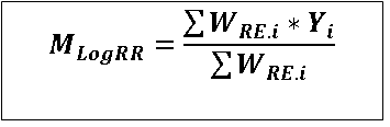
MLog OR = Summary Log OR
WRE.i= Revised weight for ith included study
Yi= Log OR for ith included study

 Standard Error of MALog OR = 1/Σ WRE.i

Once summary Log OR and its standard error is calculated, it is fairly easy to calculate confidence intervals.
We can convert summary Log OR and its confidence intervals into original scale as described above under point 4(B).

Z value and p value.

Once summary Log OR and its standard error is calculated, it is fairly easy to calculate Z value and p value using normal distribution.
Z = MALog OR / Standard Error of MALog OR

Prediction interval is calculated using following formula.


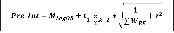
Where, t1-α/2, k-2  is (1−α/2)% percentile of t distribution with significance level α and k−2 degrees of freedom, (k = number of studies included in the meta-analysis).

Interpretation: There is a 95% (or any other specified) probability that a newly conducted study will have effect size between this interval.


Galbraith Plot

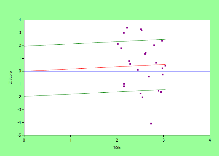
The Galbraith plot can also provide graphical representation to assess heterogeneity in the included studies.
It is a scatter plot of Z value against precision (1/SE) of each included studies. (Z value of each study = Log OR / SELog OR).
The central horizontal blue line represents the line of null effect (Log OR = 0). Studies above this line has Log OR > 0 or (Odds Ratio > 1). Studies below this line has Log OR < 0.
Middle red line represents the MA Log OR. Its slope is equal to the MA Log OR. Studies above this line has Log OR > MA Log OR. Studies below this line has Log OR < MA Log OR.
Two green line (above and below middle red line), represents the confidence intervals of MA Log OR.
In the absence of significant heterogeneity, we expect that about 95% (or other specified level) studies lie between the two green lines, and 5% (or other specified level) lie outside this. If more number of studies are outside these lines, then it indicates significant heterogeneity.
In this Galbraith plot, four studies are above the top green line and five studies are below bottom green line. So a total of 9 studies, out of 25 included studies are not within the zone bounded by two green lines, signifying heterogeneity.


Forest Plot

The forest plot represents Odds Ratio of each included study with its confidence interval. It provides collective and comprehensive graphical view of all included studies as well as Meta-analysis summary OR.
Each horizontal line represents the confidence interval of the corresponding study. Diamond at the centre on each line represents the OR reported by the study. The thickness of the diamond is proportional to the OR.
Vertical line corresponding to OR = 1, represents line of null effect. It also signifies that the studies towards left of it has shown OR < 1, whereas studies towards right has shown OR > 1. If horizontal line for any included study does not cross this vertical line, it means the corresponding study has reported significant Odds Ratio.

Forest plot also provides degree of overlap between included studies (to judge heterogeneity) and precision (as judged by the length of confidence interval) of each included study.
Bottom horizontal line with central rectangle represents MA Odds ratio and its confidence interval.
For random effects model, additional horizontal line is shown, which represents the prediction interval. It can be used to predict the results of newly conducted study. This interval tells us that about 95% (or other specified level) newly conducted studies will show effect size within this interval.


Sensitivity Analysis

The sensitivity analysis is done for each included studies by repeating meta-analysis after excluding one study at a time.
This forest plot of sensitivity analysis (one study removed) shows the MA Odds Ratio and its confidence interval, when the corresponding study is removed and MA is performed with remaining studies. In this example, the horizontal line corresponding to study MA25 (top horizontal line) shows results of Meta-analysis after study MA25 is removed and meta-analysis is performed using remaining 24 studies.
Similarly line corresponding to MA1 represents shows results of Meta-analysis after study MA1 is removed and meta-analysis is performed using remaining 24 studies.
This sensitivity analysis shows the "influence" of each included study on the original meta-analysis. If after removal of a study, the results are showing substantial change, it tells that the study has significant impact on the results of original meta-analysis,
For example, in this example, study MA11 show significant impact, as after its removal, the MA Odds Ratio has changed substantially.


Publication bias

It is a common tendency of publishers to publish "significant" studies. In other words, if result of a research is statistically non-significant, then such study can miss publication (file drawer problem). Meta-analysis includes mainly published studies, so it is often biased towards positive results. This bias is called as publication bias. The publication bias can be assessed by asymmetry of funnel plot, Begg-Mazumdar rank correlation test, Egger's regression test, Fail-Safe N, Duval and Tweedie trim and fill method.

Funnel Plot

Funnel plot is scatter plot of Effect Size (Log OR) and its Standard Error. To keep the bigger studies (with small SE) at the top, the Y axis is inverted, as shown here. So, the studies at the top are big (small SE) and studies at the bottom are small (large SE). As the studies at the bottom have large SE, to be significant they require to have larger effect size. So, the studies tend to scatter widely from top to bottom, resembling to shape of a funnel. In the absence of any publication bias, the studies are expected to spread symmetrically around central vertical line, which corresponds to the MA Log OR. In presence of significant publication bias, there will be asymmetrical spread of studies, particularly at the bottom. So, a careful assessment of the symmetry of funnel plot can tell us about the presence of publication bias.

In this example, if we look at the bottom, we can assess that around 3 or 4 "extra" studies are there to the right side. Corresponding or "mirror" studies on the left are not seen. This has caused asymmetry of the plot, suggesting presence of possible publication bias.

Note: Two other lines, on either side of central vertical lines are just guiding line to ease the assessment of asymmetry. Different softwares use different slopes for these lines, so these lines should never be used at "cut-off line" to assess asymmetry.


Begg and Mazumdar rank correlation test

Begg and Mazumdar rank correlation
Kendall's S Statistics 58
Kendall's tau without continuity correction
(* significant p value indicates significant publication bias)
Kendall's Tau 0.193
Z 1.355
p (one tailed) 0.088
Kendall's tau with continuity correction
(* significant p value indicates significant publication bias)
Kendall's Tau 0.19
Z 1.331
p (one tailed) 0.092

Funnel plot can suggest possible publication bias, but it tends to have subjective variations. Begg and Mazumdar rank correlation test can tell us objectively about the presence of publication bias. This test uses non-parametric rank correlation test based on Kendall's tau.
The power of the test is less, so significance level is often taken as twice of the intended significance level (0.1 instead of 0.05).
In this example, p value is 0.088 (without continuity correction) and 0.092 (with continuity correction). Here, p value is less than the revised significance level of 0.1 for the test, we can conclude that there is presence of significant publication bias.


Egger's regression test

Egger's regression test
(* significant p value indicates significant publication bias)
Intercept 4.51
Standard error of intercept 3.087
t value 1.461
df 23
p (one tailed) 0.0788
LB of Confidence interval -1.8763
UB of confidence interval 10.8956

Another significance test to detect publication bias is Egger's regression test. This test calculates the intercept of simple linear regression of Z score against precision (1/SE). The significant p value suggests presence of publication bias.
Here, p value is 0.0788, more than the cut-off value of 0.05.This suggests absence of significant publication bias.


Fail-Safe N (Rosenthal)

Fail-Safe N (Rosenthal)
Z value for observed studies 2.281(Fixed Effect Model)
P value for observed studies (two tailed) 0.023
Alpha 0.05
Z for given alpha (one tailed) 1.6449
Z for given alpha (two tailed) 1.96
Fail-Safe N (One tailed) 38
Fail-Safe N (Two tailed) 20

Orwin's Fail-Safe N
Effect Size in meta-analysis Odds Ratio = 1.194
Criteria for trivial effect Size
Average effect size for missing studies
Orwin's Fail-Safe N
44

Another method to assess publication bias is to calculate Fail-Safe N. We know that, publication bias is a result of non-publication of certain studies, mainly because of non-significant studies. It tends to bias the results positively or away from null effect. If we could find all such "missing" studies and add to the meta-analysis, then our meta-analysis or summary effect size will be reduced, may be to the extent that it is no more significant. But finding such "missing" or "unpublished" studies is practically not possible. Alternately we can calculate number of additional studies with average null effect required to be added to the meta-analysis to change the summary effect size to non-significant level. If such number of "missing" or "unpublished" studies, with average null effect size, required to change the p value to non-significant level, is small, then publication bias is considered. Here, we can infer that with addition of small number of possible missing or unpublished studies , the summary effect size will become non-significant. On the other hand, if such number of "missing" or "unpublished" studies are large, then safely we can conclude that there is no serious problem of publication bias. (To decide whether Fail-Safe N is small or large, it should be judiciously compared with number of studies available in the literature / included in the meta-analysis)
Classical Fail-Safe N (described by Rosenthal)
It is equal to the number of such "missing" or "unpublished" studies, with average null effect size, required to be added to the meta-analysis, to change the summary effect size to non-significant level.
In this example, the p value provided by meta-analysis is 0.023. We will need additional 20 studies, with average null effect size, to bring the p value above 0.05 (two tailed).
Orwin's Fail-Safe N
It is an alternative to classical Fail-Safe N. Classical Fail-Safe N gives number of studies required to bring down the results to non-significant level. Orwin's Fail-Safe N gives number of additional studies, required to bring down the summary effect size to a specified level (trivial criteria). Additionally, we can specify the average effect size of missing studies(M).
In this example, the summary Odds Ratio was 1.194. If trivial Odds Ratio value is considered as 1.1, and average Odds Ratio in "missing" or "unpublished" studies is taken as 1.05, then we will require 44 more such studies to be added to meta-analysis to bring down the summary Odds Ratio to 1.1. (You can change these criteria and re-calculate the Orwin's Fail-Safe N. Needless to say that, the trivial effect size criteria must be less than the MA summary effect size and average effect size must be less than trivial criteria.)


Duval and Tweedie Trim and Fill

Duval and Tweedie's Trim and Fill
Number of studies trimmed and filled Odds Ratio LB OR UB OR
Meta-analysis Results   1.194 1.025 1.39
Left sided missing studies adjusted 3 1.049 0.9071 1.2131
Right sided missing studies adjusted 0 1.194 1.025 1.39


While, all above methods of detection of publication bias can suggest or detect it, none of them gives the actual impact of probable publication bias. Trim and fill method actually detects the publication bias by detecting asymmetry of funnel plot, identifies studies that are causing asymmetry, trims (removes) those studies and finally adds these trimmed studies along with hypothetical studies which are "mirror" images of trimmed studies. Mirror image study means a hypothetical study towards the opposite side, at equivalent distance from the central MA summary measure. This will make the funnel plot symmetrical. This "fill" of mirror images is based on the consideration that these are the probable studies which are missed publication. That is why this method is called as "Trim and Fill" method. Finally, after filling of probable missed studies, meta-analysis is done again.

This revised estimate of meta-analysis, after adding hypothetical and probable missed studies, will give us the summary measure equal to what we would have got, had there was no publication bias. If the difference between original meta-analysis and after "Trim and Fill" is large, we can conclude that the impact of publication bias is significant. If the difference is minimal, we can conclude that the impact is minimal.

We will learn this method using the same funnel plot given above. The method has identified 3 studies on right side, which are causing funnel plot asymmetry. So, the method has added 3 hypothetical studies (red dots) on left side, which are mirror images of identified studies. After adding these 3 hypothetical studies, meta-analysis is revised, and revised estimates of summary measures are provided in the table. Original estimates of Odds Ratio were 1.194 (1.025 - 1.390), and revised estimates are 1.049 (0.9071 - 1.2131). Here the revised estimates are non-significant. So, we can conclude that there is significant impact of publication bias.

(The method has detected that there is no study on left side, which is causing funnel plot asymmetry. So, no study is added to the right side. So revised estimates are same as the original estimates. Funnel plot is also the same, without adding any "mirror" image study.)


Final remarks on publication bias:
In above example, Funnel plot and Begg Mazumdar test have suggested the possibility of publication bias. Whereas Egger's regression test has not suggested any significant bias. Fail-Safe N value is 38 and 44. Trim and Fill has identified publication bias and has given its possible impact.
Now, the question is how to interpret these contradictory findings?
Here, we should compare Fail-Safe N with number of available studies in meta-analysis(38 or 44 versus 25). When, 25 studies are detected by our search, is it possible to have another ~ 40 "missing" studies? The answer is, it may be, especially when the effect size is minimal.
Secondly, "Trim and Fill" has shown that, if 3 "missing" studies are added, the effect size will be non-significant. This is the most important factor for final interprtation. If, the results of MA are changing like this, we should consider significant publication bias.
On the contrary, even if publication bias is detected, but its impact is minimal, we can just mention its presence and safely ignore it.


L'abb´e Plot

The L’Abb´e plot is a scatterplot of the log odds in the controls and cases group on the x axis and the y axis, respectively. (Odds = number of exposed / number of non-exposed) The log odds are plotted as circles with their sizes proportional to study size or precision (1/SE).
The central thin pink reference line is the line of similar outcomes in control and case group. If a study has equal log odds in controls and cases, the circle corresponding to this study will lie on this line. If a study has larger log odds for cases than controls, then the circle will lie above the line. If a study has larger log odds for controls than cases, then the circle will lie below the line.
The other line represents estimated overall effect-size line. This plot can be used to explore heterogeneity by outlying studies. How?
It is expected that, all the studies will follow the overall effect-size line. Studies far away from this line suggest heterogeneity. Additionally, as the sizes of circles represent the study size (or precision), we can have an idea about "pull" phenomenon caused by such large study.
In this L'abb´e plot, there are few studies away from the overall effect-size line, suggesting heterogeneity.

If available data is in the form of OR and its confidence interval, then we do not have odds in cases and controls. So, L'abb'e plot can not be generated.


@ Sachin Mumbare